Trump Voters in Winsconsin
The research question of interest involves the factors influencing voters in Winsconsin to vote for Trump in the 2016 U.S. election. In this research, we are mainly interested in demographic factors such as race and rurality. It is hypothesized that there exists an urban/rural and racial phenomenon for Trumpism; such that Trump appealed to White voters and areas with low population density in 2016, with significant spatial variation.
A Besag York Mollié Bayesian Hierarchical Spatial Model
In order to fit a statistically robust model that quantifies the problem, data collected from the 2016 election results in Winsconsin, as collected and published on Harvard Dataverse, were used to analyze the profile of Trump voters in Winsconsin. Scraped data in .RData format can also be downloaded in my github repo.
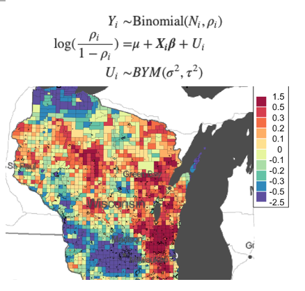
We chose to run the model on the sub-county level because county level data is too aggregated to find significant results and census tract level data is too detailed and create unnecessary noises. As we are interested in finding spatial variations in Trump supporter along with some demographic factors, a bayesian spatial model BYM with binomial distribution was constructed using diseasemapping R package to fit the data, as displayed below:
\[ \begin{aligned} Y_{i} \sim & \text{Binomial}(N_{i}, \rho_{i})\\ \text{log}(\frac{\rho_{i}}{1-\rho_{i}}) = & \mu + \boldsymbol{X_{i}\beta} + U_i\\ U_i \sim& BYM(\sigma^2, \tau^2) \end{aligned} \]
# BYM model with sensible priors
resTrump2 = diseasemapping::bym(
  trump ~ logPdens + propWhite + propInd,
  data = wisconsinCsubm,
  priorCI = list(
              sd = c(0.5, 0.05),
               propSpatial = c(0.2, 0.5)),
  Ntrials = wisconsinCsubm$Total,
  family = "binomial")
\(Y_i\) represents the number of Trump voters, \(N_i\) represents the total number of voters, and \(\rho_i\) is the probability they vote for Trump. For each region, the logit probability depends on covariates \(X_i\beta\) and random effect \(U_i\), \(\mu\) being the intercept. The random effect \(U_i\) consists two standard diviation parameters: spatial (\(\sigma^2\)) and independent (\(\tau^2\)). \(X_i\) is a vector of covariates including proportion of residents in the sub-county who are white (porpWhite), proportion of residents in the sub-county who are Indigenous (propInd), and population density (logPdens). Population density factor was scaled using log() in order to be on the same scale as the other covariates.
Penalized complexity priors were chosen for standard deviation, which includes both non-spatial and spatial parameters, as c(0.5, 0.05), meaning the probability of standard deviation is bigger than 0.5 is 5%. And the penalized complexity prior for spatial proportion (propSpatial) is c(0.2, 0.5), meaning the median of the spatial proportion is 0.2, assuming a rougher surface than it is smooth. Prior for \(\beta\) was left at INLA default. We chose the above prior distribution to encourage the model to be boring and surface to be flat; by doing so, we can learn truly from the data whether there is anything significantly correlated.
Results
Log Lative Risk and Odds Ratios Tables
# log relative risk (logged odds ratios) table
temp <- resTrump2$parameters$summary[,c(1,3,5)]
table1 <- temp %>%
  kableExtra::kbl(
    caption = "Figure 1. Parameter Posterior Means and 95% Credible Intervals
    (Log Odds)", booktabs = T, digits = 3) %>%
  kableExtra::kable_classic(full_width = F, html_font = "Cambria") %>%
  kableExtra::kable_styling(latex_options = c("HOLD_position", "striped"))

# odds ratios table
logOddsMat = resTrump2$parameters$summary[,c(4,3,5)]
oddsMat = exp(logOddsMat)
oddsMat[1,] = oddsMat[1,]/(1 + oddsMat[1, ])
rownames(oddsMat)[1] = 'Baseline prob'
table2 <- oddsMat %>%
  kableExtra::kbl(
    caption = "Figure 2. BYM Model Results From Voting Data (Odds Ratio)",
    booktabs = T, digits = 3) %>%
  kableExtra::kable_classic(full_width = F, html_font = "Cambria") %>%
  kableExtra::kable_styling(latex_options = c("HOLD_position", "striped"))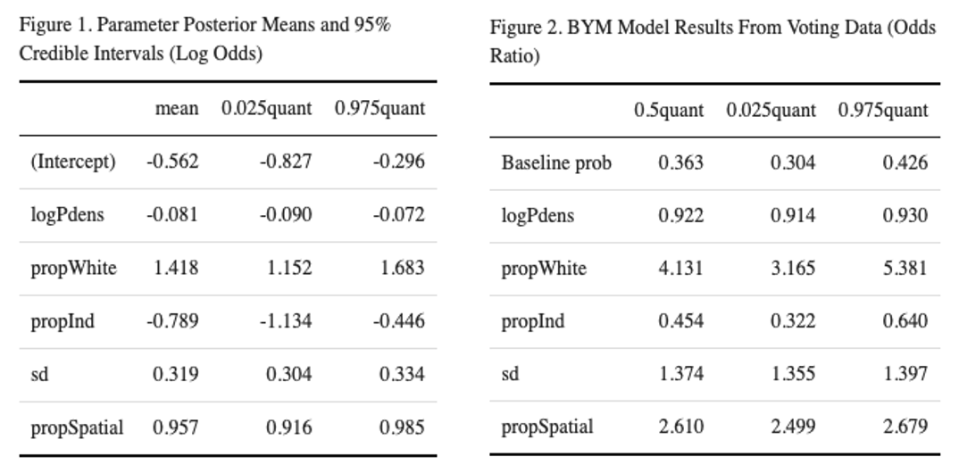
Table 1 shows the parameter posterior means and 95% credible intervals in logged odds ratios. This table provides valuable information on the significance of variables. If the mean is equal to, or the credible interval includes, 0, the corresponding variable is not significant. From this table, we can conclude that population density and proportion of indigenous people in a sub-county have significant negative correlation with Trump votes turnout, while proportion of white people in a sub-county level is strongly correlated with Trump votes turnout in a positive way. The overall standard deviation is 0.32, and most of the variance is being explained by the spatial proportion, around 96%. There is a strong spatial effect for Trump voters in Winsconsin.
Table 2 is the IQR version of table 1, displaying the parameters in odds ratio. We can conclude that a 1% increase in the proportion of white residents on the sub-county level will result in a 4.1% increase in Trump votes, or a 3.2 - 5.4% increase with 95% confidence interval. A 1% increase in the proportion of indigenous residents only result in a 0.45% increase in Trump votes and a 1 standard deviation increase in population density results in a 0.92% increase in Trump votes. Figure 1 and 2 display the prior and posterior density distribution for overall standard deviation and spatial proportion.
Prior and Posterior Distributions
# prior and posteriors for SD
plot(resTrump2$parameters$sd$posterior, type = 'l', xlim = c(0,1),
     xlab = 'sd', ylab = 'dens',
     main = 'Figure 1. Prior and Posterior Distribution for Standard Deviation',
     cex.main = 0.6)
lines(resTrump2$parameters$sd$prior, col = 'grey')
legend('topright', lty = 1, col = c('black', 'grey'),
       legend = c('post', 'prior'), bty = 'n')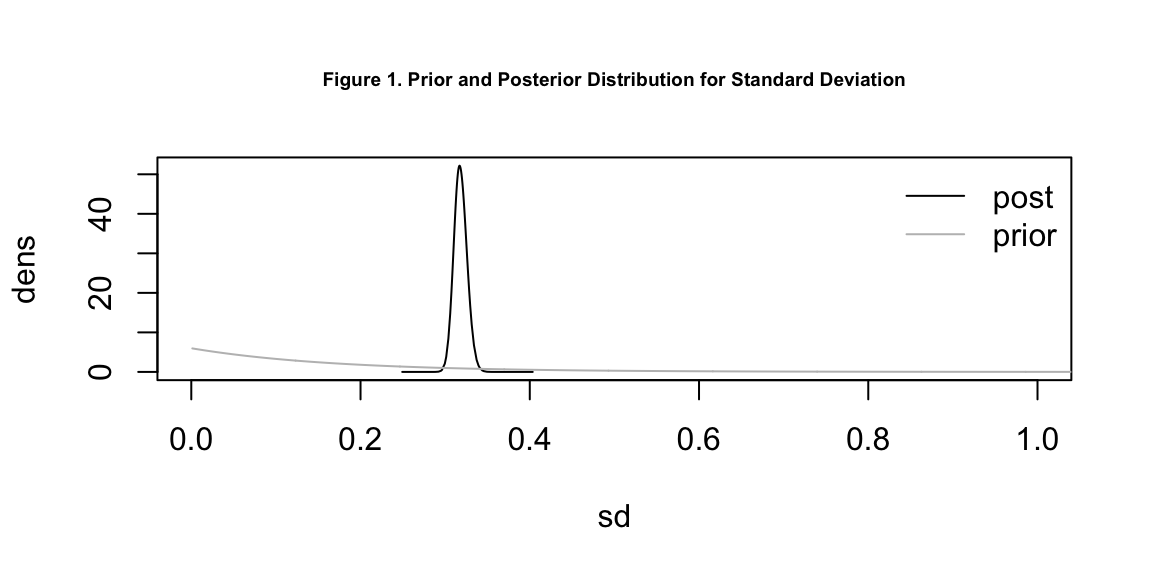
# prior and posterior for spatial proportion
plot(resTrump2$parameters$propSpatial$posterior, type = 'l', xlim = c(0,2.5),
     xlab = 'prop spatial', ylab = 'dens',
     main = 'Figure 2. Prior and Posterior Distribution for Spatial Proportion',
     cex.main = 0.6)
lines(resTrump2$parameters$propSpatial$prior, col = 'red')
legend('topright', lty = 1, col = c('black', 'red'),
       legend = c('post', 'prior'), bty = 'n')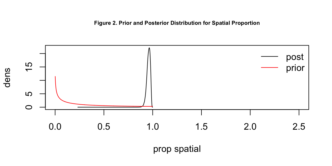
Random Effect and Exceedance Probability Maps
theColTrump = mapmisc::colourScale(wisconsinCsubm$propTrump, col = "RdBu",
                                   breaks = sort(
                                     unique(setdiff(
                                       c(0, 1,seq(0.2,0.8, by = 0.1)), 0.5))),
                                   style = "fixed", rev = TRUE)
theColPop = mapmisc::colourScale(wisconsinCsubm$pdens,
                                 col = "Spectral",
                                 breaks = 11, style = "equal",
                                 transform = "log", digits = 1,rev = TRUE)
theColWhite = mapmisc::colourScale(wisconsinCsubm$propWhite,
                                   col = "Spectral",
                                   breaks = c(0, 0.5, 0.8, 0.9,
                                              seq(0.9, 1, by = 0.02)),
                                   style = "fixed", rev = TRUE)
theColInd = mapmisc::colourScale(wisconsinCsubm$propInd,
                                 col = "Spectral", breaks = seq(0, 1, by = 0.1),
                                 style = "fixed", rev = TRUE)
theBg = mapmisc::tonerToTrans(
  mapmisc::openmap(wisconsinCm, fact = 2, path = "stamen-toner"),
  col = "grey30")
theInset = mapmisc::openmap(wisconsinCm, zoom = 6, path = "stamen-watercolor",
                            crs = mapmisc::crsMerc,
                            buffer = c(0, 1500, 100, 700) *1000)

theColRandom = mapmisc::colourScale(resTrump2$data$random.mean,
                                    col = "Spectral", breaks = 11,
                                    style = "quantile", rev = TRUE, dec = 1)
theColFit = mapmisc::colourScale(resTrump2$data$fitted.invlogit, col = "RdBu",
                                 rev = TRUE,
                                 breaks = sort(unique(setdiff(
                                   c(0,1,seq(0.2, 0.8, by = 0.1)),0.5))),
                                 style = "fixed")

# plot
mapmisc::map.new(wisconsinCsubm, 0.85)
plot(resTrump2$data, col = theColRandom$plot, add = TRUE, lwd = 0.2)
plot(theBg, add = TRUE, maxpixels = 10^7)
mapmisc::legendBreaks("topright", theColRandom)
title(main = 'Figure 3. Random Effect Map', line = -1.5)

mapmisc::map.new(wisconsinCsubm, 0.85)
plot(resTrump2$data, col = theColFit$plot, add = TRUE, lwd = 0.2)
plot(theBg, add = TRUE, maxpixels = 10^7)
mapmisc::legendBreaks("topright", theColFit)
title(main = 'Figure 4. Exceedance Probability Map ', line = -1.5)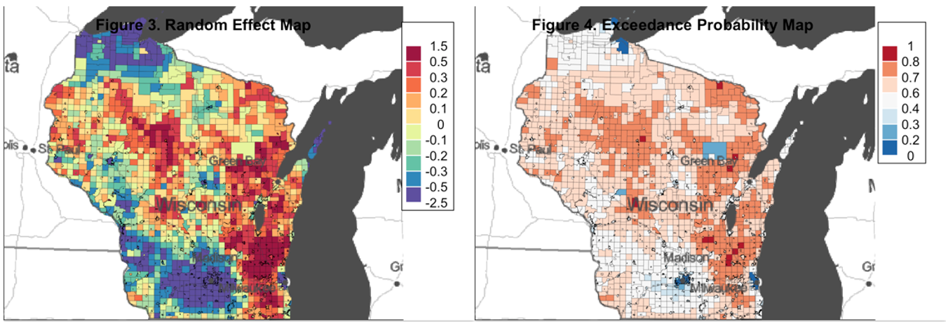
Figure 3 and 4 are the random effect map and exceedance probability map, respectively. In figure 3, red areas indicate regions with large uncertainty. The variations in these regions cannot be explained properly by covariates (urban/rural and racial profile), indicating large random effects. Since there are a lot of uncertainty in figure 3, figure 4- the exceedance probability map displays the probability that the random effect is causing more than 1/4th of excess Trump voting. We know that there is excess Trump voting for areas in red, there is no excess Trump voting for areas in blue, and we are unsure for the areas in color that are in between.
Discussion
Overall, demographic factors such as population density, proportion of white or indigenous people on sub-county level, as well as spatial effect are significant with Trump votes turnout in Wisconsin for the 2016 U.S. election. Regions with a greater proportion of residents who are white result in an increase in the proportion of Trump votes. In contrasts, regions with greater of residents who are indigenous or with higher population density result in a decrease in the proportion of Trump votes. There are also a great amount of variation explained by the spatial effect, meaning areas closer together are likely to have similar proportion of Trump votes.
Maggie Ma
Aspiring Data Scientist & Geospatial Analyst
My interests include predictive modeling, machine learning, spatial statistics, and data visualization.